
One of the pains I often hear about is the lack of ‘out-of-the-box’ functionality in Tableau that allows you to restrict what values are displayed in Quick Filters. This ability would be extremely useful when you don’t want the values excluded in calculations / view, but just want to exclude it as a filter display i.e. so that your users won’t be able to click on it. At my current client site, I needed to do exactly that (plus allow my users to select multiple values in the filter “multi-select”).
Today’s blog is all about how to achieve just that. I’ll be talking about 3 different techniques of restricting filter values, however bear in mind that only the 1st technique met all of my requirements and thus is the one I ended up using. The 2nd and 3rd techniques are there as alternative options for those of you out there who don’t have as specific a requirement; I’ll also be talking about their drawbacks.
Let’s assume I’m building a dashboard where I’m comparing the measure values for Regions (Americas, Asia and Europe). The measure values span across three years (2017, 2018 and 2019), but I don’t want my users clicking on ‘2017’ (thus I’m going to exclude that value from being displayed at all in the filter dropdown). That is not to say I don’t still want 2017 values being included in any calculations or views however! For example, if I were to select ‘All’, I’d still expect the total to comprise of 2017, 2018 and 2019 records.
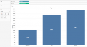
Before I delve into the techniques, I’ve included a Reference screenshot to check back against; this is the total measure value for each of the Regions without the ‘Financial Year’ filter applied. When my users click on ‘(All)’ financial years, these are the numbers they should be seeing.
Reference screenshot:
Let the tale begin….
This technique involves duplicating the Financial Year dimension in a dummy worksheet before bringing that worksheet into the dashboard itself.
First, duplicate the Financial Year dimension.
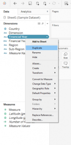
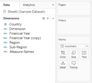
Open up a new worksheet and give it a name. I’m going to call it ‘Filter display sheet’. Drop both ‘Financial Year’ and ‘Financial Year (copy)’ to the Filters shelf, making sure all its values are selected, and show filter.
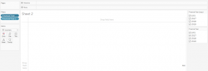
Then on the ‘Financial Year (copy)’ filter, untick the value you want to exclude (in this case ‘2017’). On the original ‘Financial Year’ filter, select “Only Relevant Values”.
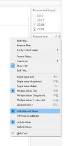
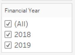
Your original filter will now look like this, as it has now adopted the values you’ve selected (or rather, didn’t select) in the duplicate filter:
Now comes the crucial step. Drag your ‘Filter display sheet’ onto the dashboard (you’ll need to hide the title as this acts as a ‘dummy’ worksheet so it shouldn’t be visible). This step is to ensure that it now has access to the original Financial Year filter with 2017 ‘excluded’.
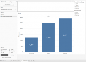
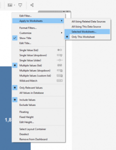
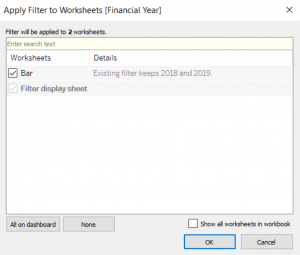
Remove ‘Financial Year (copy)’ from the dashboard and on the ‘Financial Year’ carrot dropdown, hover over “Apply to worksheets”, click on “Selected Worksheets” and click on “Bar” to ensure the filter now also controls the Bar graph visual.

Your view should now look like this:
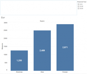
What you’ll notice about this technique is that even though ‘2017’ is excluded as a value from the quick filter, its numbers are not excluded in the calculation (compare this to ‘Reference screenshot’ at the top). Furthermore notice that you can use this filter as a multi-select.
If you were to repeat the same process on the worksheet “Bar” instead of on another dummy worksheet, then it will exclude 2017 values altogether.
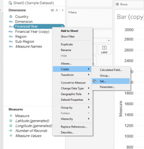
An alternative way of restricting filter values is by way of Sets. Right click on ‘Financial Year’ to create a Set:
Select only 2018 and 2019 in the Set before depositing it into Filters shelf. Now you can use the Set as a filter; right click on the set and “Show Filter”.
Disclaimer:
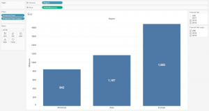
What you’ll immediately notice with Sets is that by excluding 2017 from the filter dropdown, you have also excluded the values from the calculation (view) itself hence why the numbers are less than the equivalent screenshot for Filters above. There’s nothing wrong with using Sets if excluding it from the calculation is what you intended to do!
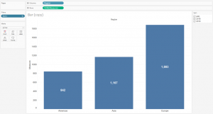
Right click on blank space in the Data pane to “Create Parameter”. Select the Data type as ‘String’ and type up the values you intend to display in your make-shift filter:
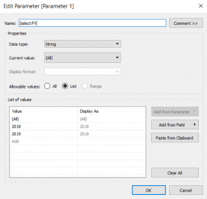
Show the parameter by right clicking, “Show Parameter Control”.
Link the parameter by dropping the ‘Financial Year’ dimension into the filters shelf. Select the “Condition” tab, select “By formula” and link the parameter with your quick filter as per the equation boxed in purple below:
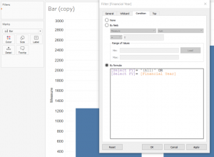
Now what you’ll find is that the parameter behaves like the Filters technique in that when you select ‘(All)’ it doesn’t exclude the 2017 value from the calculation (view) even though it is excluded as a display.
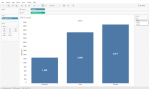
Disclaimer:
However, with parameters, you’ll notice that you cannot use it as a ‘multi-select’ unfortunately.
In summary, you can apply any of the 3 techniques above as long as it’s fit for your purpose. But in short, if you want to:
a. Exclude a value from filter display
b. Not exclude the value from the actual calculation (view); and
c. Allow users to use it as a multi-dropdown;
Then safe to say that Technique 1. is your best bet.
I hope you found this article useful! Stay tuned for more tips and tricks!
If you would like me to send you the tableau packaged workbook, please email me at ana.yin@tridant.com.au.
Copyright © Tridant Pty Ltd.